Train `PINN`#

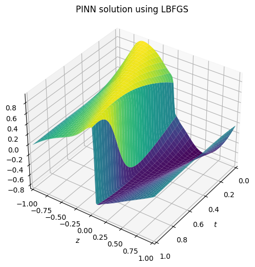
In this example, physics informed neural network (PINN) technique is used to train burgers equation.

Physics-Informed Neural Networks (PINNs) use physical rules or equations in their architecture or loss function. This enables them learn from data and respect the physical laws governing the modeled system.

Many traditional machine learning models focus primarily on dataset fitting. This works for many applications, but it may not be enough if the system being investigated has physical laws to follow. Models with physically unreasonable predictions may result from ignoring these rules.

PINNs add a term to the loss function to ensure that neural network predictions obey differential equations, boundary conditions, or other physical rules.

In the following tutorial, simple PINN network is to be trained with adam optimizer from optax package, and LBFGS optimizer from jaxopt package.

Imports#

[1]:

!pip install git+https://github.com/ASEM000/serket --quiet
!pip install optax --quiet
!pip instal jaxopt --quiet  # for second-order optimizers

ERROR: unknown command "instal" - maybe you meant "install"

[2]:

import jax
import jax.numpy as jnp
import jax.random as jr
import matplotlib.pyplot as plt
import matplotlib as mpl
from matplotlib import cm
import optax
import jaxopt
import serket as sk

Equation#

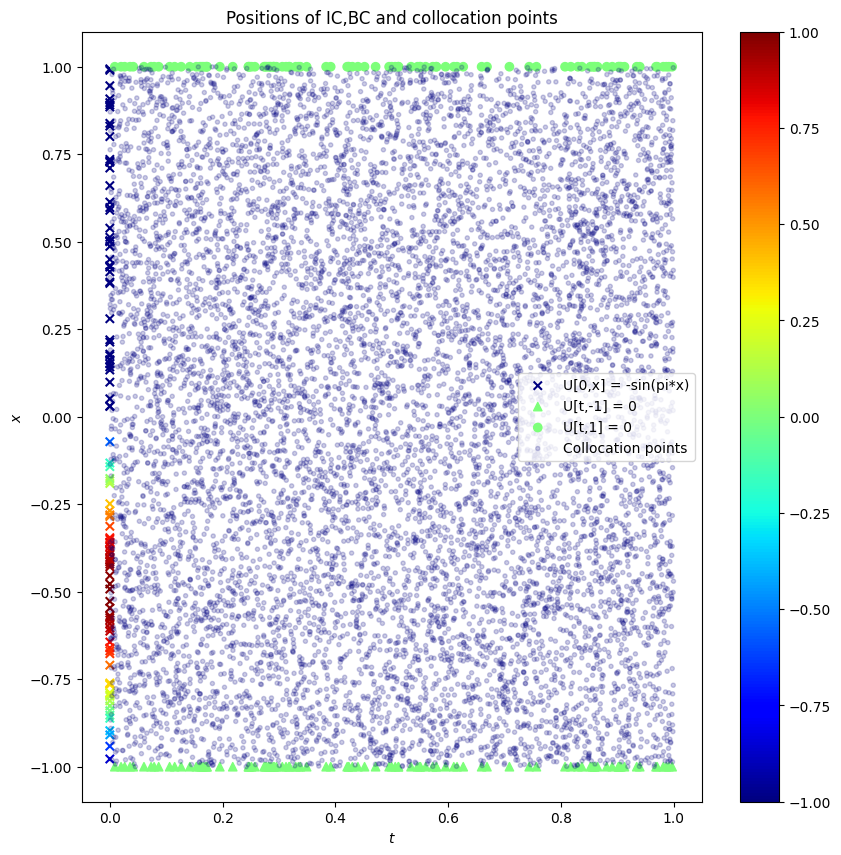
\[\begin{aligned} \partial_t u + u \, \partial_x u - (0.01/\pi) \, \partial_{xx} u &= 0, \quad &&\quad (t,x) \in (0,1] \times (-1,1),\\ u(0,x) &= - \sin(\pi \, x), \quad &&\quad x \in [-1,1],\\ u(t,-1) = u(t,1) &= 0, \quad &&\quad t \in (0,1]. \end{aligned}\]

Data preparation#

[3]:

N_0 = 100  # number of points for initial condition
N_b = 100  # number of points for boundary condition
N_r = 10_000  # number of points for collocation

tmin, tmax = 0.0, 1.0
xmin, xmax = -1.0, 1.0

"""boundary conditions"""

keys = jax.random.split(jax.random.key(0), 5)

# u[0,x] = -sin(pi*x)
t_0 = jnp.ones([N_0, 1], dtype="float32") * 0.0
x_0 = jr.uniform(key=keys[0], minval=xmin, maxval=xmax, shape=(N_0, 1))
ic_0 = -jnp.sin(jnp.pi * x_0)

# U[t,-1] = 0
t_b1 = jr.uniform(key=keys[1], minval=tmin, maxval=tmax, shape=(N_b, 1))
x_b1 = jnp.ones_like(t_b1) * -1
bc_1 = jnp.zeros_like(t_b1)

# U[t,1] = 0
t_b2 = jr.uniform(key=keys[1], minval=tmin, maxval=tmax, shape=(N_b, 1))
x_b2 = jnp.ones_like(t_b2)
bc_2 = jnp.zeros_like(t_b2)

# collocation points
t_c = jr.uniform(key=keys[2], minval=tmin, maxval=tmax, shape=(N_r, 1))
x_c = jr.uniform(key=keys[3], minval=xmin, maxval=xmax, shape=(N_r, 1))
z_c = jnp.zeros_like(t_c)

Data visualization#

[4]:

fig, ax = plt.subplots(figsize=(10, 10))
ax.scatter(
    t_0,
    x_0,
    c=ic_0,
    marker="x",
    vmin=0,
    vmax=1,
    label="U[0,x] = -sin(pi*x)",
    cmap=cm.jet,
)
ax.scatter(
    t_b1,
    x_b1,
    c=bc_1,
    marker="^",
    vmin=-1,
    vmax=1,
    label="U[t,-1] = 0",
    cmap=cm.jet,
)
ax.scatter(
    t_b2,
    x_b2,
    c=bc_2,
    marker="o",
    vmin=-1,
    vmax=1,
    label="U[t,1] = 0",
    cmap=cm.jet,
)


cmap = mpl.cm.jet
norm = mpl.colors.Normalize(vmin=-1, vmax=1)


ax.scatter(
    t_c,
    x_c,
    c=jnp.zeros_like(t_c),
    marker=".",
    alpha=0.2,
    label="Collocation points",
    cmap=cm.jet,
)


ax.set_xlabel("$t$")
ax.set_ylabel("$x$")

ax.set_title("Positions of IC,BC and collocation points")
plt.colorbar(mpl.cm.ScalarMappable(norm=norm, cmap=cmap))
plt.legend(loc="center right")

/var/folders/mv/cckpw89s2jjd622p9pywk0nm0000gn/T/ipykernel_53501/1429392938.py:53: MatplotlibDeprecationWarning: Unable to determine Axes to steal space for Colorbar. Using gca(), but will raise in the future. Either provide the *cax* argument to use as the Axes for the Colorbar, provide the *ax* argument to steal space from it, or add *mappable* to an Axes.
  plt.colorbar(mpl.cm.ScalarMappable(norm=norm, cmap=cmap))

[4]:

<matplotlib.legend.Legend at 0x14b05f810>

../_images/notebooks_%5Bguides%5D%5Btrain%5Dpinn_burgers_8_2.png

Define the neural network#

In this step, we define a neural network \(NN\) to satisfy the following equations

\[\begin{aligned} \partial_t NN_u + NN_u \, \partial_x NN_u - (0.01/\pi) \, \partial_{xx} NN_u &= 0, \quad &&\quad (t,x) \in (0,1] \times (-1,1),\\ NN_u(0,x) &= - \sin(\pi \, x), \quad &&\quad x \in [-1,1],\\ NN_u(t,-1) = NN_u(t,1) &= 0, \quad &&\quad t \in (0,1]. \end{aligned}\]

[5]:

class PINN(sk.TreeClass):
    def __init__(self, key: jax.Array):
        keys = jr.split(key, 5)
        self.linear1 = sk.nn.Linear(2, 8, key=keys[0])
        self.linear2 = sk.nn.Linear(8, 8, key=keys[1])
        self.linear3 = sk.nn.Linear(8, 8, key=keys[2])
        self.linear4 = sk.nn.Linear(8, 8, key=keys[3])
        self.linear5 = sk.nn.Linear(8, 1, key=keys[4])

    def __call__(self, t: jax.Array, x: jax.Array) -> jax.Array:
        z = jnp.concatenate([t, x], axis=-1)
        z = jnp.tanh(self.linear1(z))
        z = jnp.tanh(self.linear2(z))
        z = jnp.tanh(self.linear3(z))
        z = jnp.tanh(self.linear4(z))
        z = self.linear5(z)
        return z

Define the loss function#

[6]:

def sum_func(func):
    return lambda *args: jnp.sum(func(*args))


def mse(x: jax.Array, y: jax.Array) -> jax.Array:
    assert x.shape == y.shape
    return jnp.mean((x - y) ** 2)


def loss_func(net: PINN) -> jax.Array:
    net = sk.tree_unmask(net)  # unmask the network parameters
    loss = mse(net(t_0, x_0), ic_0)  # initial condition loss
    loss += mse(net(t_b1, x_b1), bc_1)  # boundary condition loss
    loss += mse(net(t_b2, x_b2), bc_2)  # boundary condition loss

    # pde loss
    net_x = jax.grad(sum_func(net), 1)
    net_xx = jax.grad(sum_func(net_x), 1)
    net_t = jax.grad(sum_func(net), 0)

    lhs = net_t(t_c, x_c) + net(t_c, x_c) * net_x(t_c, x_c)
    rhs = (0.01 / jnp.pi) * net_xx(t_c, x_c)
    loss += mse(lhs, rhs)

    return loss

Define `adam` train step#

In this step, adam optimizer from optax is used to train.

[7]:

pinn = PINN(key=jr.key(0))

# mask the network parameters to use it across jax transformations
pinn = sk.tree_mask(pinn)

print(sk.tree_summary(pinn, depth=1))

lr = optax.piecewise_constant_schedule(
    init_value=1e-2,
    boundaries_and_scales={10_000: 0.1},
)
optim = optax.adam(lr)
optim_state = optim.init(pinn)


@jax.jit
def train_step(net: PINN, optim_state: optax.OptState):
    loss, grads = jax.value_and_grad(loss_func)(net)
    updates, optim_state = optim.update(grads, optim_state)
    net = optax.apply_updates(net, updates)
    return net, optim_state, loss


for i in range(1, 20_000 + 1):
    pinn, optim_state, loss = train_step(pinn, optim_state)
    if i % 500 == 0:
        print(f"Step {i:005d} loss {loss:.3e} lr {lr(i):.3e}")

# finally unmask the network parameters to use it
pinn = sk.tree_unmask(pinn)

┌────────┬──────┬─────┬───────┐
│Name    │Type  │Count│Size   │
├────────┼──────┼─────┼───────┤
│.linear1│Linear│24   │96.00B │
├────────┼──────┼─────┼───────┤
│.linear2│Linear│72   │288.00B│
├────────┼──────┼─────┼───────┤
│.linear3│Linear│72   │288.00B│
├────────┼──────┼─────┼───────┤
│.linear4│Linear│72   │288.00B│
├────────┼──────┼─────┼───────┤
│.linear5│Linear│9    │36.00B │
├────────┼──────┼─────┼───────┤
│Σ       │PINN  │249  │996.00B│
└────────┴──────┴─────┴───────┘
Step 00500 loss 1.093e-01 lr 1.000e-02
Step 01000 loss 6.875e-02 lr 1.000e-02
Step 01500 loss 4.410e-02 lr 1.000e-02
Step 02000 loss 5.203e-02 lr 1.000e-02
Step 02500 loss 6.511e-03 lr 1.000e-02
Step 03000 loss 5.114e-03 lr 1.000e-02
Step 03500 loss 4.435e-03 lr 1.000e-02
Step 04000 loss 4.016e-03 lr 1.000e-02
Step 04500 loss 3.603e-03 lr 1.000e-02
Step 05000 loss 7.565e-03 lr 1.000e-02
Step 05500 loss 3.148e-03 lr 1.000e-02
Step 06000 loss 2.852e-03 lr 1.000e-02
Step 06500 loss 8.434e-03 lr 1.000e-02
Step 07000 loss 2.504e-03 lr 1.000e-02
Step 07500 loss 2.174e-03 lr 1.000e-02
Step 08000 loss 2.517e-03 lr 1.000e-02
Step 08500 loss 2.774e-03 lr 1.000e-02
Step 09000 loss 2.252e-03 lr 1.000e-02
Step 09500 loss 1.323e-03 lr 1.000e-02
Step 10000 loss 1.770e-03 lr 1.000e-03
Step 10500 loss 1.137e-03 lr 1.000e-03
Step 11000 loss 1.116e-03 lr 1.000e-03
Step 11500 loss 1.094e-03 lr 1.000e-03
Step 12000 loss 1.069e-03 lr 1.000e-03
Step 12500 loss 1.042e-03 lr 1.000e-03
Step 13000 loss 1.012e-03 lr 1.000e-03
Step 13500 loss 9.788e-04 lr 1.000e-03
Step 14000 loss 9.419e-04 lr 1.000e-03
Step 14500 loss 9.028e-04 lr 1.000e-03
Step 15000 loss 8.681e-04 lr 1.000e-03
Step 15500 loss 8.352e-04 lr 1.000e-03
Step 16000 loss 8.059e-04 lr 1.000e-03
Step 16500 loss 8.316e-04 lr 1.000e-03
Step 17000 loss 7.551e-04 lr 1.000e-03
Step 17500 loss 7.612e-04 lr 1.000e-03
Step 18000 loss 8.238e-04 lr 1.000e-03
Step 18500 loss 7.176e-04 lr 1.000e-03
Step 19000 loss 6.729e-04 lr 1.000e-03
Step 19500 loss 6.553e-04 lr 1.000e-03
Step 20000 loss 6.384e-04 lr 1.000e-03

Plot results#

[8]:

N = 100
tspace = jnp.linspace(tmin, tmax, N + 1)
xspace = jnp.linspace(xmin, xmax, N + 1)
T, X = jnp.meshgrid(tspace, xspace)
U = pinn(T.flatten().reshape(-1, 1), X.flatten().reshape(-1, 1)).reshape(N + 1, N + 1)

fig = plt.figure(figsize=(9, 6))
ax = fig.add_subplot(111, projection="3d")
ax.plot_surface(T, X, U, cmap=cm.viridis)
ax.set_xlim(tmin, tmax)
ax.set_ylim(xmin, xmax)
ax.view_init(35, 35)
ax.set_xlabel("$t$")
ax.set_ylabel("$z$")
ax.set_title("PINN solution using ADAM")

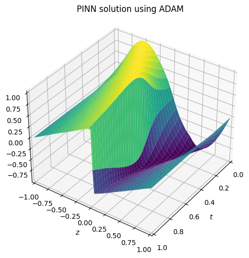
[8]:

Text(0.5, 0.92, 'PINN solution using ADAM')

../_images/notebooks_%5Bguides%5D%5Btrain%5Dpinn_burgers_16_1.png

Define `LBFGS` train step#

In this step jaxopt library LBFGS optimizer is used to train for the network.

[9]:

pinn = PINN(key=jr.key(0))

# mask the network parameters to use it across jax transformations
pinn = sk.tree_mask(pinn)

print(sk.tree_summary(pinn, depth=1))

# note that loss function is only passed to the optimizer
pinn = sk.tree_unmask(jaxopt.LBFGS(fun=loss_func).run(pinn).params)
# we can continue training with ADAM
# similar to the step above. for this guide we skip it.

┌────────┬──────┬─────┬───────┐
│Name    │Type  │Count│Size   │
├────────┼──────┼─────┼───────┤
│.linear1│Linear│24   │96.00B │
├────────┼──────┼─────┼───────┤
│.linear2│Linear│72   │288.00B│
├────────┼──────┼─────┼───────┤
│.linear3│Linear│72   │288.00B│
├────────┼──────┼─────┼───────┤
│.linear4│Linear│72   │288.00B│
├────────┼──────┼─────┼───────┤
│.linear5│Linear│9    │36.00B │
├────────┼──────┼─────┼───────┤
│Σ       │PINN  │249  │996.00B│
└────────┴──────┴─────┴───────┘

Plot results#

[10]:

N = 100
tspace = jnp.linspace(tmin, tmax, N + 1)
xspace = jnp.linspace(xmin, xmax, N + 1)
T, X = jnp.meshgrid(tspace, xspace)
U = pinn(T.flatten().reshape(-1, 1), X.flatten().reshape(-1, 1)).reshape(N + 1, N + 1)

fig = plt.figure(figsize=(9, 6))
ax = fig.add_subplot(111, projection="3d")
ax.plot_surface(T, X, U, cmap=cm.viridis)
ax.set_xlim(tmin, tmax)
ax.set_ylim(xmin, xmax)
ax.view_init(35, 35)
ax.set_xlabel("$t$")
ax.set_ylabel("$z$")
ax.set_title("PINN solution using LBFGS")

[10]:

Text(0.5, 0.92, 'PINN solution using LBFGS')

../_images/notebooks_%5Bguides%5D%5Btrain%5Dpinn_burgers_20_1.png

Train PINN

Contents

Train `PINN`#

Imports#

Equation#

Data preparation#

Data visualization#

Define the neural network#

Define the loss function#

Define `adam` train step#

Plot results#

Define `LBFGS` train step#

Plot results#

Train PINN

Contents

Train PINN#

Imports#

Equation#

Data preparation#

Data visualization#

Define the neural network#

Define the loss function#

Define adam train step#

Plot results#

Define LBFGS train step#

Plot results#

Train `PINN`#

Define `adam` train step#

Define `LBFGS` train step#